How to Calculate CTC Loss of DL Model in PyTorch?

PyTorch is the framework with the torch module containing the functions and dependencies in the Python language. The combination of Python and torch forms the name PyTorch which is used to design Artificial Intelligence models with Machine Learning or Deep Learning. Evaluating these models is an important phase that comes after the training process and PyTorch offers multiple loss functions for that.

Finding loss using statistical formulas can be vital and considered an evaluation technique that compares the input values with the predicted values. The loss is evaluated for the predicted values by checking how much it differs from the actual input provided during the training. Connectionist Temporal Classification or CTC Loss maps the probabilities of the predicted tensors on the input probabilities.

Quick Outline

This guide explains the following sections:

• What is CTC Loss
• How to Calculate CTC Loss of DL Model in PyTorch
• Conclusion

What is CTC Loss

The Connectionist Temporal Classification (CTC) loss function can be used when we need to find an alignment between multiple sequences which is a challenging task. One of the major applications of CTC loss will be aligning each character and placing it in its correct location with the soundtrack. It simply produces a loss value to find the difference of each node by summing probabilities of alignments in the input and the target sequences.

How to Calculate CTC Loss of DL Model in PyTorch

The CTC loss function can be used to evaluate the performance of the deep learning models. The user can train these models with multiple iterations learning insights of the data. With each iteration, the model starts to improve its performance and the loss value starts to decrease. To calculate the CTC loss of the DL model in PyTorch, simply go through the following steps:

Note: The Python code to calculate the CTC loss is available here

Step 1: Access Python Notebook

Open a new Python project in Google Colab to execute the Python code and it can be accessed from the official website:

Step 2: Install Modules & Import Libraries

On the notebook, start the code by installing the JiWER package from the pip package manager using the following code. The JiWER is the Python package to compute the performance of the ML or DL model for speech recognition applications using Word Error Rate(WER) and others:

pip install jiwer

After that, import the required libraries to make the environment ready for building and training the deep learning model. The following code contains the list of all the possible needed libraries to evaluate and plot graphs of the model’s performance:

import matplotlib.pyplot as pltimport pandas as pdimport numpy as npimport tensorflow as tffrom tensorflow import kerasfrom IPython import displayfrom jiwer import werfrom tensorflow.keras import layers

Step 3: Loading the DataSet

Now that the libraries are imported successfully, download the data from the provided URL or use the data that you have to train the model on. This is called the input data which can be used by the model to get hidden patterns and learn to understand its complexities to predict accurately:

data_url = "https://data.keithito.com/data/speech/LJSpeech-1.1.tar.bz2"
data_path = keras.utils.get_file("LJSpeech-1.1", data_url, untar=True)
wavs_path = data_path + "/wavs/"
metadata_path = data_path + "/metadata.csv"
#The dataset contains the metadata of the input for the model
metadata_df = pd.read_csv(metadata_path, sep="|", header=None, quoting=3)
metadata_df.columns = ["file_name", "transcription", "normalized_transcription"]#store the file’s name and the normalized form of data in the file
metadata_df = metadata_df[["file_name", "normalized_transcription"]]
metadata_df = metadata_df.sample(frac=1).reset_index(drop=True)
metadata_df.head()

The above code:

• data_url variable contains the link to download the data from the internet in the tar format
• The data_path stores the root directory that contains the data for the model
• The wavs_path variable contains the data_path and the waves folder with the audio files
• The data also has the metadata for the model that tells the insights about the data and makes the job easier for the model and is stored in the metadata_path variable
• Build the data frames using the pandas as pd to read the downloaded dataset and integrate it with the model
• Define the metadata_df.columns to store the names of the field from the data set and it can be used to filter the noise from the data
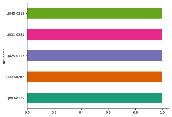
• After loading the dataset to the colab session, simply print the head() method to displays top 5 rows of the dataset:

The following picture displays the files from the head() with their files_name and duration of the audio file to understand the length of the data:

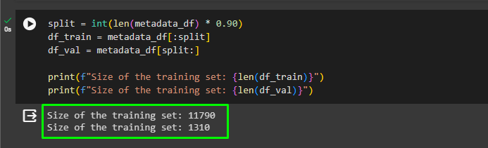
Step 4: Splitting Data into Training & Testing Data

Once the data set is loaded to the session and we know its orientation, it’s time to split it into training and testing data. The training data is the only data that will be given to the model for its training and understanding of the complexities. Once the model is trained, we will give the testing data which is unseen for the model, and get the predictions using the testing data. This process will tell us how good the model is performing on the unseen data and if it’s good enough for the world or not:

split = int(len(metadata_df) * 0.90)
df_train = metadata_df[:split]
df_val = metadata_df[split:]
#printing the number of instances in the training and testing data
print(f"Size of the training set: {len(df_train)}")
print(f"Size of the training set: {len(df_val)}")

• The split variable takes the length of the complete data and takes the 90 percent and gives it to the df_train variable.
• The remaining 10 percent will be stored in the df_test variable and used as the testing data to check the model’s performance.
• Once the data is split into two sets, simply print the number of files stored in both sets:

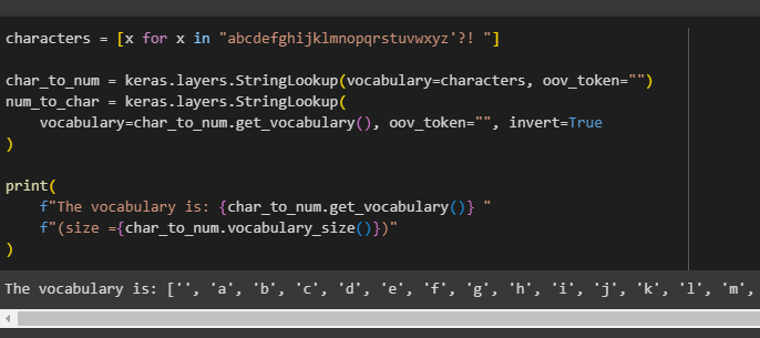
Step 5: Setting up Vocabulary

Now, the model has no idea about the language used in the audio files so we need to provide some context of the language. For that, define the characters variable and use the for loop to store the English alphabets using the following code:

characters = [x for x in "abcdefghijklmnopqrstuvwxyz'?! "]

char_to_num = keras.layers.StringLookup(vocabulary=characters, oov_token="")
num_to_char = keras.layers.StringLookup(
    vocabulary=char_to_num.get_vocabulary(), oov_token="", invert=True
)
#The alphabets stored in the vocabulary using the get_vocabulary function
print(
    f"The vocabulary is: {char_to_num.get_vocabulary()} "
    f"(size ={char_to_num.vocabulary_size()})"
)

The code:

• Stores the English alphabets in the characters variable using the loop
• Defines two variables named char_to_num for getting the numbers for the string and then the num_to_char for understanding the characters using the numbers assigned to them.
• At the end, it code returns the characters stored in the vocabulary and their size as well:

Step 6: Normalizing the Data

Now it’s time to configure the intermediate steps that normalize the data which enables the model to work efficiently:

frame_length = 256
frame_step = 160
fft_length = 384

def encode_single_sample(wav_file, label):
    file = tf.io.read_file(wavs_path + wav_file + ".wav")
    audio, _ = tf.audio.decode_wav(file)
    audio = tf.squeeze(audio, axis=-1)
    audio = tf.cast(audio, tf.float32)
    spectrogram = tf.signal.stft(
        audio, frame_length=frame_length, frame_step=frame_step, fft_length=fft_length
    )
#The normalization of the audio file with their frame_length and steps
    spectrogram = tf.abs(spectrogram)
    spectrogram = tf.math.pow(spectrogram, 0.5)
    means = tf.math.reduce_mean(spectrogram, 1, keepdims=True)
    stddevs = tf.math.reduce_std(spectrogram, 1, keepdims=True)#The spectrogram subtracted by its mean and divided by the SD
    spectrogram = (spectrogram - means) / (stddevs + 1e-10)
    label = tf.strings.lower(label)
    label = tf.strings.unicode_split(label, input_encoding="UTF-8")
    label = char_to_num(label)
    return spectrogram, label

The code:

• Explains the sample audio file and then uses the read_file() method to read the audio files. 
• It also comprises the files and converts the audio file into the spectrogram using tf.signal.stft() method
• At the end, it simply returns the normalized version of the spectrogram which can be applied to the complete dataset for building a speech recognition system:

After normalizing the dataset, apply the normalization to the training and testing datasets by storing them in the train_dataset and validation_dataset variables. The encode_single_sample() is applied on all the files using the map() method and num_parralel_calls run in parallel for the efficiency of the model:

batch_size = 32
train_dataset = tf.data.Dataset.from_tensor_slices(
    (list(df_train["file_name"]), list(df_train["normalized_transcription"]))
)
train_dataset = (
    train_dataset.map(encode_single_sample, num_parallel_calls=tf.data.AUTOTUNE)
    .padded_batch(batch_size)
    .prefetch(buffer_size=tf.data.AUTOTUNE)
)

validation_dataset = tf.data.Dataset.from_tensor_slices(
    (list(df_val["file_name"]), list(df_val["normalized_transcription"]))
)
validation_dataset = (
    validation_dataset.map(encode_single_sample, num_parallel_calls=tf.data.AUTOTUNE)
    .padded_batch(batch_size)
    .prefetch(buffer_size=tf.data.AUTOTUNE)
)

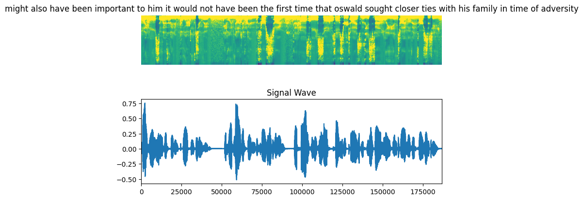
Execute the following code to plot the waveform visualization for the spectrogram using the 8 x 5 graph on the training data:

fig = plt.figure(figsize=(8, 5))
for batch in train_dataset.take(1):#using for loop to take the audio files from the dataset and plot their wavegraphs
    spectrogram = batch[0][0].numpy()
    spectrogram = np.array([np.trim_zeros(x) for x in np.transpose(spectrogram)])
    label = batch[1][0]
    label = tf.strings.reduce_join(num_to_char(label)).numpy().decode("utf-8")
    ax = plt.subplot(2, 1, 1)
    ax.imshow(spectrogram, vmax=1)
    ax.set_title(label)
    ax.axis("off")
    file = tf.io.read_file(wavs_path + list(df_train["file_name"])[0] + ".wav")
    audio, _ = tf.audio.decode_wav(file)
    audio = audio.numpy()
    ax = plt.subplot(2, 1, 2)
    plt.plot(audio)
    ax.set_title("Signal Wave")
    ax.set_xlim(0, len(audio))
    display.display(display.Audio(np.transpose(audio), rate=16000))
plt.show()

The above code returns the sample audio file with its string and signal wave representation as displayed in the following snippet:

Step 7: Configure CTCLoss() Method

After normalizing the data, define the CTCLoss() method to find the loss value from the input and predicted values. The CTCLoss() method is generally used to evaluate all the models but its performance is improved in the speech recognition problem:

def CTCLoss(y_true, y_pred):
    batch_len = tf.cast(tf.shape(y_true)[0], dtype="int64")#set the input and label length variables to compare the shapes of the original and predicted strings
    input_length = tf.cast(tf.shape(y_pred)[1], dtype="int64")
    label_length = tf.cast(tf.shape(y_true)[1], dtype="int64")
    input_length = input_length * tf.ones(shape=(batch_len, 1), dtype="int64")
    label_length = label_length * tf.ones(shape=(batch_len, 1), dtype="int64")

    loss = keras.backend.ctc_batch_cost(y_true, y_pred, input_length, label_length)
    return loss

Step 8: Building the Neural Network Model

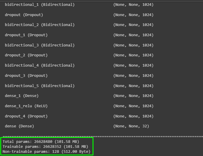
Configure the deep learning model by defining the build_model() method with the dimensions and layers as the arguments. The deep learning or neural network model to be specific works in multiple layers with neurons present in each layer connected to the next layer. It forms a network to transmit signals from the first layer to the other while training the model to get the final output:

#building the model using the RNN model with the layers and neuronsdef build_model(input_dim, output_dim, rnn_layers=5, rnn_units=128):
    """Model very close to DeepSpeech2"""
    input_spectrogram = layers.Input((None, input_dim), name="input")#setup the first layer of the neural network model
    x = layers.Reshape((-1, input_dim, 1), name="expand_dim")(input_spectrogram)
    x = layers.Conv2D(
        filters=32,
        kernel_size=[11, 41],
        strides=[2, 2],
        padding="same",
        use_bias=False,
        name="conv_1",
    )(x)#set up the second layer of the neural network model
    x = layers.BatchNormalization(name="conv_1_bn")(x)
    x = layers.ReLU(name="conv_1_relu")(x)
    x = layers.Conv2D(
        filters=32,
        kernel_size=[11, 21],
        strides=[1, 2],
        padding="same",
        use_bias=False,
        name="conv_2",
    )(x)#set up the third layer of the neural network model
    x = layers.BatchNormalization(name="conv_2_bn")(x)
    x = layers.ReLU(name="conv_2_relu")(x)
    x = layers.Reshape((-1, x.shape[-2] * x.shape[-1]))(x)
    for i in range(1, rnn_layers + 1):
        recurrent = layers.GRU(
            units=rnn_units,
            activation="tanh",
            recurrent_activation="sigmoid",
            use_bias=True,
            return_sequences=True,
            reset_after=True,
            name=f"gru_{i}",
        )#set up the bi-directional model for the backpropagation to improve the accuracy
        x = layers.Bidirectional(
            recurrent, name=f"bidirectional_{i}", merge_mode="concat"
        )(x)
        if i < rnn_layers:
            x = layers.Dropout(rate=0.5)(x)
#adding the dimensions and activation functions to the neurons and layers
    x = layers.Dense(units=rnn_units * 2, name="dense_1")(x)
    x = layers.ReLU(name="dense_1_relu")(x)
    x = layers.Dropout(rate=0.5)(x)
    output = layers.Dense(units=output_dim + 1, activation="softmax")(x)
   model = keras.Model(input_spectrogram, output, name="DeepSpeech_2")
    opt = keras.optimizers.Adam(learning_rate=1e-4)
    model.compile(optimizer=opt, loss=CTCLoss)
    return model
#integrate the components and store it in a single variable
model = build_model(
    input_dim=fft_length // 2 + 1,
    output_dim=char_to_num.vocabulary_size(),
    rnn_units=512,
)
model.summary(line_length=110)

The code:

• Builds the network with 5 layers and then configures each layer with its neurons and activation functions.
• The Recurrent Neural Network or RNN model is being configured which is built to understand the speech and convert it into text for the user.
• At the end, it displays the summary of the model as displayed in the below screenshot:

Step 9: Training the Model

Train the model by configuring the intermediate steps that a model should perform to go through the input data by defining the decode_batch_prediction() method:

def decode_batch_predictions(pred):
    input_len = np.ones(pred.shape[0]) * pred.shape[1]#decode the predictions to the strings in human language for human understanding
    results = keras.backend.ctc_decode(pred, input_length=input_len, greedy=True)[0][0]
    output_text = []
    for result in results:
        result = tf.strings.reduce_join(num_to_char(result)).numpy().decode("utf-8")
        output_text.append(result)
    return output_text

class CallbackEval(keras.callbacks.Callback):
    """Shows the outputs using batch for every iteration"""

    def __init__(self, dataset):
        super().__init__()
        self.dataset = dataset
#defining the process when the iteration ends with the value of the loss and accuracy
    def on_epoch_end(self, epoch: int, logs=None):
        predictions = []
        targets = []
        for batch in self.dataset:
            X, y = batch#body of the for loop to store the predictions in batches
            batch_predictions = model.predict(X)
            batch_predictions = decode_batch_predictions(batch_predictions)
            predictions.extend(batch_predictions)#loop for the predicted labels
            for label in y:
                label = (
                    tf.strings.reduce_join(num_to_char(label)).numpy().decode("utf-8")
                )
                targets.append(label)
        wer_score = wer(targets, predictions)
        print("-" * 100)
        print(f"Loss: {wer_score:.4f}")
        print("-" * 100)#loop to print the target and predictions for each iteration
        for i in np.random.randint(0, len(predictions), 2):
            print(f"Target    : {targets[i]}")
            print(f"Prediction: {predictions[i]}")
            print("-" * 100)

The above code:

• It enables the model to go through the complete dataset in one iteration and returns how much it understood by providing the sample predictions.
• The sample predictions take the input data and the model tries to replicate it and keeps on growing with each iteration.
• At the start, the loss value is 1 meaning that the model knows nothing but with epochs, it starts learning and the loss value goes down.
• It uses the Word Error Rate from the JiWER package to return the error value as well:

The following code configures the number of iterations for the model and the validation callbacks to fit the model on the dataset:

epochs = 5

validation_callback = CallbackEval(validation_dataset)
history = model.fit(
    train_dataset,
    validation_data=validation_dataset,
    epochs=epochs,
    callbacks=[validation_callback],
)

The following screenshot display the performance of the model after 5 iterations and it can be improved with more iterations as well:

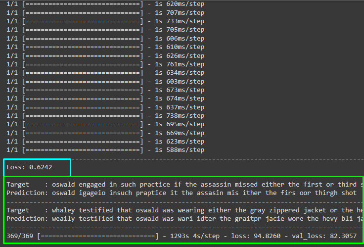
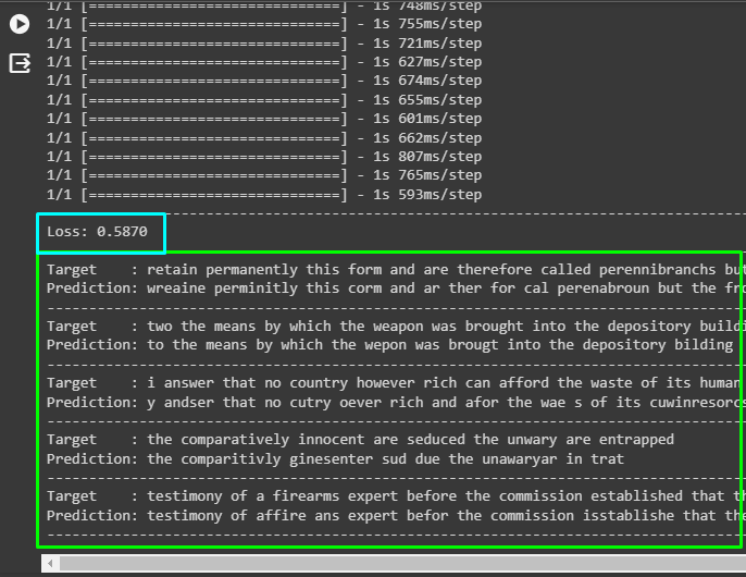
Step 10: Testing the Model

Finally, it’s time to test the performance of the model after 5 iterations, to get the predictions using the unseen audio files. The batch_predictions variable contains the predict() method that enables the model to start predicting the strings from the audio:

predictions = []
targets = []
for batch in validation_dataset:
    X, y = batch
    batch_predictions = model.predict(X)#storing and extending the batch predictions
    batch_predictions = decode_batch_predictions(batch_predictions)
    predictions.extend(batch_predictions)
    for label in y:
        label = tf.strings.reduce_join(num_to_char(label)).numpy().decode("utf-8")
        targets.append(label)
wer_score = wer(targets, predictions)
print("-" * 100)
print(f"Loss: {wer_score:.4f}")
print("-" * 100)#loop to print the target and predictions for each iteration
for i in np.random.randint(0, len(predictions), 5):
    print(f"Target    : {targets[i]}")
    print(f"Prediction: {predictions[i]}")
    print("-" * 100)

The following screenshot displays that the loss value is about 59% followed by the 5 strings that the model predicted. The predictions are not completely accurate but the models have done a pretty good job with that and some more training will make it more effective:

That’s all about how to calculate the CTC loss of the DL model in PyTorch.

Conclusion

To calculate the CTC loss value from the deep learning model, train the neural network model and train it using the input data that is accurate. After that, define the CTCLoss() class to get the loss value of the trained model which enables us to observe the model’s accuracy. The loss value can also be used to enhance the performance of the model using more training. This guide has elaborated on how to calculate the CTC loss value of the trained deep learning model.