
PyTorch is the framework that can be used to build deep learning models in Python programming language to get accurate predictions. The machine is usually taught through some historical dataset containing actual values as the input. It is better to get the dataset with a variety of values and hidden patterns so the machine takes the time to understand every detail inside it.
Quick Outline
This guide explains the following sections:
- What is the Confusion Matrix?
- What are the Dice Similarity Coefficient and Dice Loss?
- How to Calculate Dice Loss of DL Model in PyTorch
What is the Confusion Matrix?
It is important to understand the concept of the confusion matrix before getting to know the Dice loss or any other loss function. The confusion matrix gives an overall view of all the predictions from the dataset and makes it easy to understand the model’s performance. The user can simply evaluate or test the performance of the model by looking at the data from the confusion matrix:
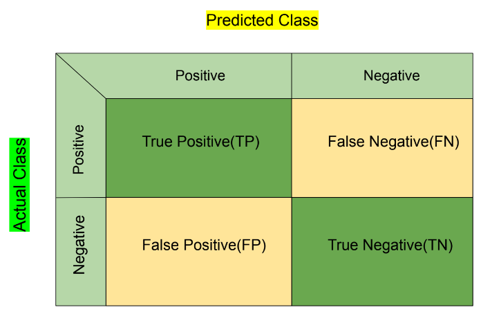
We take the actual values of the dataset on the Y-axis(Vertical) and the predicted values across the X-axis(Horizontal) each with the classes. The True Positive(TP) box contains the values that were positive in the actual dataset and the model predicted them as positives. The same for the True Negative(TN) as they are the negative values in actual and predicted fields. The False Negative(FN) are the initial positive values, and the model predicted them as negative. Actual negative values that are predicted as positive are called False Positive(FP) in the confusion matrix:
| Input Values | Predicted Values | Labels |
|---|---|---|
| Positive | Positive | True Positive(TP) |
| Positive | Negative | False Negative(FN) |
| Negative | Positive | False Positive(FP) |
| Negative | Negative | True Negative(TN) |
Add all the values from each class and place the values in the confusion matrix to apply different formulas for evaluation.
Before understanding or implementing the Dice Loss, it is important to understand the Dice Similarity Coefficient or DSC. The next section explains the DSC and the Dice loss in detail with the mathematical representations:
What are the Dice Similarity Coefficient and Dice Loss?
The Dice Similarity Coefficient or DSC can be extracted from the confusion matrix using its values and then the Dice loss will be extracted automatically. The Dice Loss and the Dice Similarity Coefficient are the inverse of each other and finding one will automatically discover the other. The following is the mathematical representation of the Dice Similarity Coefficient:
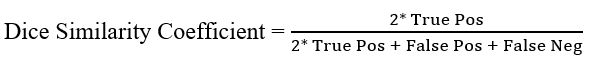
The DSC formula takes the true positive values from the dataset and multiplies it by 2 to place it as the numerator. After that, take the numerator and store it as the denominator after adding the false values for the positive and negative classes.
Once the DSC value is calculated, simply subtract it by 1 to take its inverse value which will be considered as the Dice loss:

How to Calculate Dice Loss of DL Model in PyTorch
Deep learning models can be evaluated using the Dice loss by plotting the true or false values on the confusion matrices. Firstly, build and train the neural network model with multiple iterations to understand the hidden patterns in the data. The loss functions are to enhance the performance of the deep learning model and the following steps explain its implementation:
Note: The Python code for the examples can be accessed from here:
Step 1: Accessing Python Notebook
Open the Python notebook by clicking the “New Notebook” button from the Google Colaboratory page. The user can also use other notebooks like Jupyter to write the code in Python language:

Step 2: Importing Libraries
In the colab notebook, import the libraries to build the deep learning model and define the loss function which is dice for this guide. Use multiple iterations to improve the predictions of the model and end the process by plotting the values of the model on the confusion matrix:
import torch
from torch import Tensor as tf
import tensorflow as tf
import numpy as np
import seaborn as sns
import matplotlib.pyplot as plt
from sklearn.metrics import confusion_matrix
Step 3: Customizing the Dice Loss Function
Define the dice_loss() with the actual and predicted values of the data in the argument and return the loss value:
def dice_loss(y_true, y_pred):
    smooth = 1.0
    intersection = tf.reduce_sum(y_true * y_pred)
    union = tf.reduce_sum(y_true) + tf.reduce_sum(y_pred)
    dice_coefficient = (2.0 * intersection + smooth) / (union + smooth)
    loss = 1.0 - dice_coefficient
    return loss
The code:
- Defines the dice_loss() method and its components to build the formula to calculate the loss value
- Before calculating the dice loss value, we need to calculate the dice_coefficient using the intersection, smooth, and union variables.
- Once the dice_coefficient is calculated, simply get the loss value by subtracting 1 from it:
Step 4: Building the MLP Model
As the loss function is ready, simply use it in the Multi-layered Perceptron or MLP model which consists of completely connected layers. The neural network model contains the neuron stored in the layers and the neurons of one layer are connected to the next layer in the network. In the MLP model, there are 3 layers in which one is hidden and each neuron is connected to all the neurons from the next layer:
def create_mlp(input_dim, num_classes):
    model = tf.keras.models.Sequential([
        tf.keras.layers.Dense(64, activation='relu', input_dim=input_dim),
        tf.keras.layers.Dense(64, activation='relu'),
        tf.keras.layers.Dense(num_classes, activation='softmax')
    ])
    return model

input_dim = 100
num_classes = 10
mlp_model = create_mlp(input_dim, num_classes)
mlp_model.summary()
mlp_model.compile(loss=dice_loss, optimizer='adam', metrics=['accuracy'])
The code:
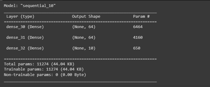
- Defines the create_mlp() method with the dimensions and number of classes of the DL model.
- Build the model using the sequential() method defining three layers with 64 neurons in the first 2 layers which are the input and hidden layers.
- The last layer is the output layer which contains one neuron in the sequential model and all the layers use the activation function.
- The activation function from each layer is used to take the input from the previous layer and apply some functions using the weights and biases to calculate the output for the next layer.
- Once the model is created, simply store it in the mlp_model to compile it using the loss function and display the summary of the model:
Step 5: Training the Model
After configuring the model, start the training process which means that the model goes through the data set multiple times to learn its complexities. The training is done using an epoch or iteration that takes the input from the dataset and applies the activation functions for each layer to get the output value at the end:
train_data = np.random.random((1000, input_dim))
train_labels = np.random.randint(num_classes, size=(1000, 1))

train_labels_one_hot = tf.keras.utils.to_categorical(train_labels, num_classes)
mlp_model.fit(train_data, train_labels_one_hot, epochs=10, batch_size=32)
test_data = np.random.random((100, input_dim))
predictions = mlp_model.predict(test_data)
predicted_labels = np.argmax(predictions, axis=1)

print(predicted_labels)
The code:
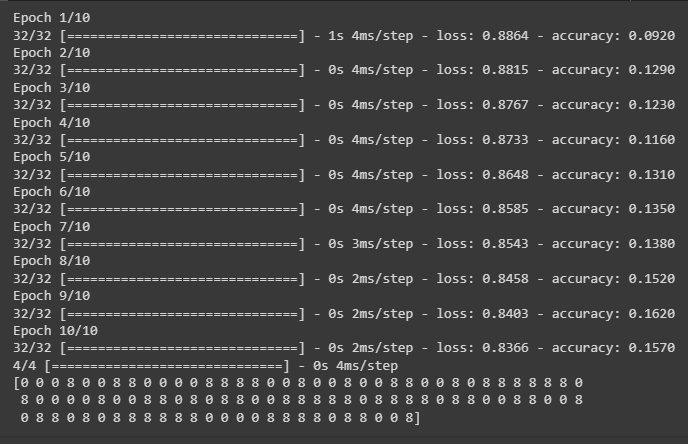
- Takes the dataset using the numpy library and stores it in the train_data variable with their labels for the confusion matrix.
- Also, train the model using the fit() method with the number of epochs and batch_size for each iteration as displayed in the following screenshot.
- After that, test the model using the predictions made by the model with the loss and accuracy value for each iteration.
- Each iteration improves the model performance by minimizing the loss value and raises the accuracy:
Step 6: Plotting the Model’s Performance
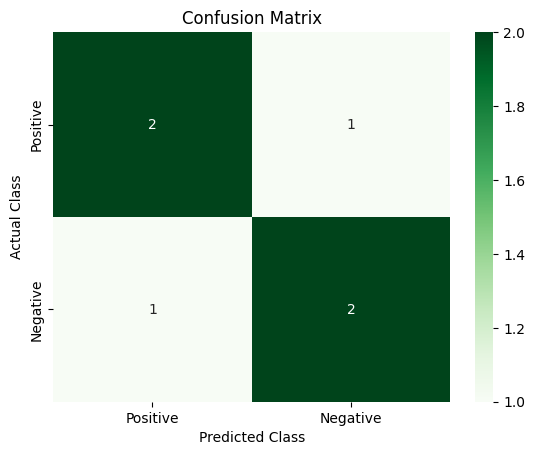
Finally, visually represent the performance of the model by plotting the values on the confusion matrix using accurate and predicted classes:
true_labels = np.array([1, 1, 0, 1, 0, 0])
predicted_labels = np.array([1, 0, 0, 1, 0, 1])
cm = confusion_matrix(true_labels, predicted_labels)

class_labels = ['Positive', 'Negative']
sns.heatmap(cm, annot=True, cmap='Greens', fmt='d', xticklabels=class_labels, yticklabels=class_labels)

plt.xlabel("Predicted Class")
plt.ylabel("Actual Class")
plt.title("Confusion Matrix")

plt.show()- Get the true and predicted labels from the dataset and call the confusion_matrix() method in the cm variable.
- Set the names for the rows and columns to place the actual and predicted values in the matrix.
- Build the confusion matrix using the heatmap() method to build a two_dimensional representation with the arguments like cm for the confusion matrix.
- The annot argument is used to place the values on its designated cell and the cmap argument sets the different shades of the color for the cells.
- The fmt argument is used to select the data type of the values to be stored in the matrix and d stands for the decimal.
- Finally displays the confusion matrix on the screen as displayed in the following picture:
That’s all about the Dice Similarity Coefficient and its loss with the implementation.
Conclusion
To calculate the dice loss value of the deep learning model, import the libraries in the Python notebook to use their functions in Python language. Define the formula for the Dice Loss function in the dice_loss() method and use it while building the MLP model. After that, train the model with multiple epochs with the values of loss and accuracy of each iteration. In the end, design the confusion matrix to display the values for each cell using a graphical representation. This guide has elaborated on the process of calculating the dice loss of the deep learning model in PyTorch.
Frequently Asked Questions
What is the importance of understanding the Confusion Matrix in deep learning models?
Understanding the Confusion Matrix is crucial as it provides an overall view of the model's performance by comparing actual and predicted values.
How does the Confusion Matrix help in evaluating the performance of a machine learning model?
The Confusion Matrix helps in evaluating the model's performance by highlighting True Positive, True Negative, False Positive, and False Negative values.
What role does the Dice Similarity Coefficient play in deep learning models?
The Dice Similarity Coefficient measures the similarity between two samples and is commonly used in image segmentation tasks.
How can the Dice Loss function benefit the training of deep learning models in PyTorch?
The Dice Loss function helps in optimizing deep learning models by penalizing false positives and false negatives, improving segmentation accuracy.
Why is it important to calculate Dice Loss in PyTorch for model training?
Calculating Dice Loss in PyTorch is crucial for assessing model performance and improving the accuracy of segmentation tasks in deep learning.
What are the key steps involved in calculating Dice Loss of a deep learning model in PyTorch?
To calculate Dice Loss in PyTorch, one needs to compute the Dice coefficient, dice numerator, and dice denominator for accurate model evaluation.
How does PyTorch facilitate the calculation of Dice Loss for deep learning models?
PyTorch provides efficient tools and functions to calculate Dice Loss, making it easier for developers to optimize their deep learning models.
Can the Dice Loss metric be used for other types of machine learning models apart from deep learning?
While Dice Loss is commonly used in deep learning for segmentation tasks, it can also be applied to other machine learning models for performance evaluation.