
Cells are the building blocks of Google Sheets that store all the data. Google Sheets has very useful customizing tools to make the data in the cells more understandable. In this guide, we will learn how we can customize the formatting of cells in Google Sheets to make our spreadsheet more pleasant and clear.
How to Format Cells in Google Sheets?
Formatting cells in Google Sheets like changing text style, size and color, especially when you have large data in Google Sheets, makes it more visible and easier to understand. There are many ways by which we can format the cells in Google Sheets, we will discuss each of them one by one.
Most of the formatting options are available on the toolbar in Google Sheets as follows:
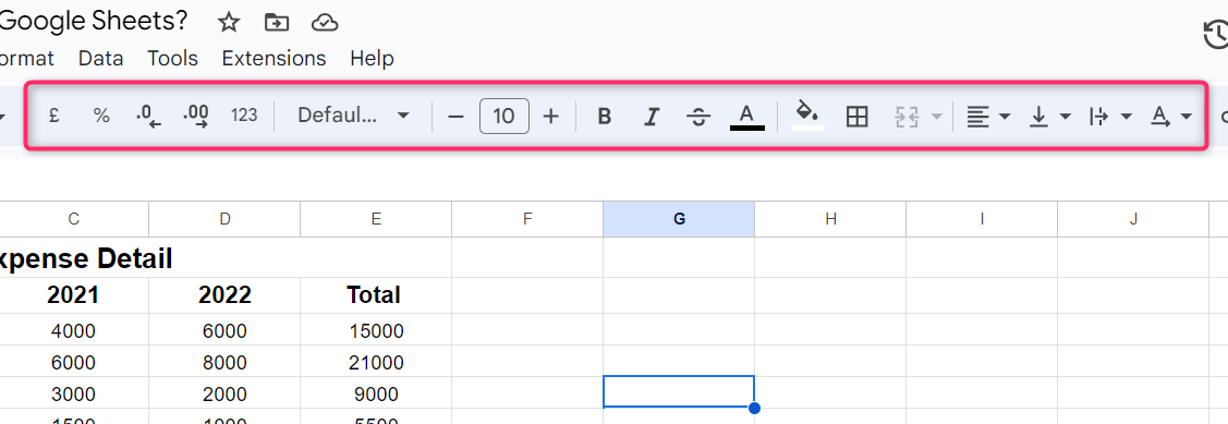
Now, we will discuss all the formatting tools one by one as follows.
- How to Format Cells by Changing Font Style
- How to Format Cells by Changing Font Size
- How to Format Cells by Changing Font Color
- How to Format Cells by Changing Fill Color
- How to Format Cells by Typographical Emphasis
- How to Format Cells by Changing Cell Sizes
- How to Format Cells by Adding Cell Borders
- How to Format Cells by Data Formatting in Cells
How to Format Cells by Changing Font Style
There are multiple font style options available in Google Sheets. To change the font style in Google Sheets, follow the following steps.
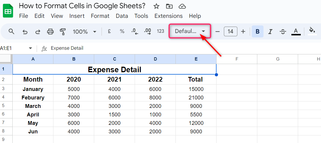
Step 1: Select Cells
Select the cells on which you want to change the font style and click on the box under Default (Arial) in the toolbar. By default, the font style in Arial style:
Step 2: Select Font Style
Select the font style from the dropdown to apply to the selected cells:
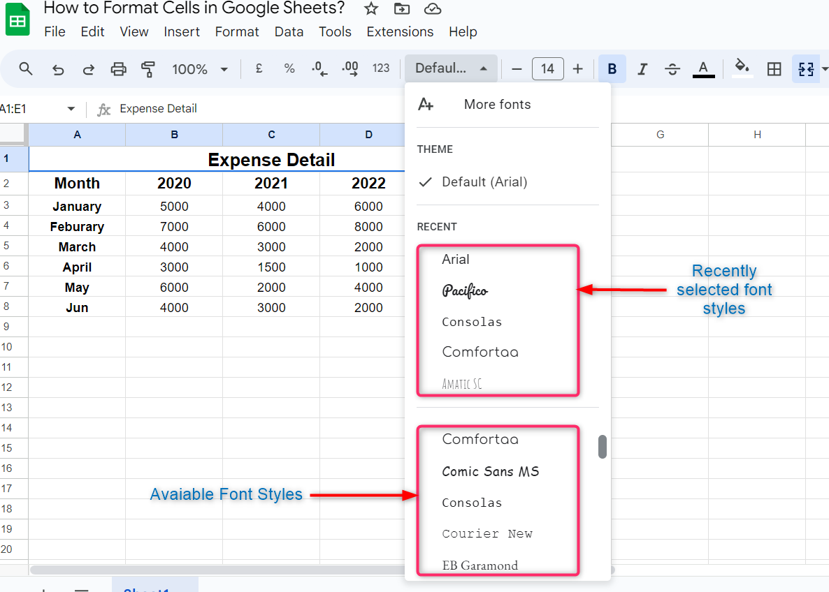
If the font style you wish to apply is not available in the dropdown, then click on More fonts at the top of the dropdown:
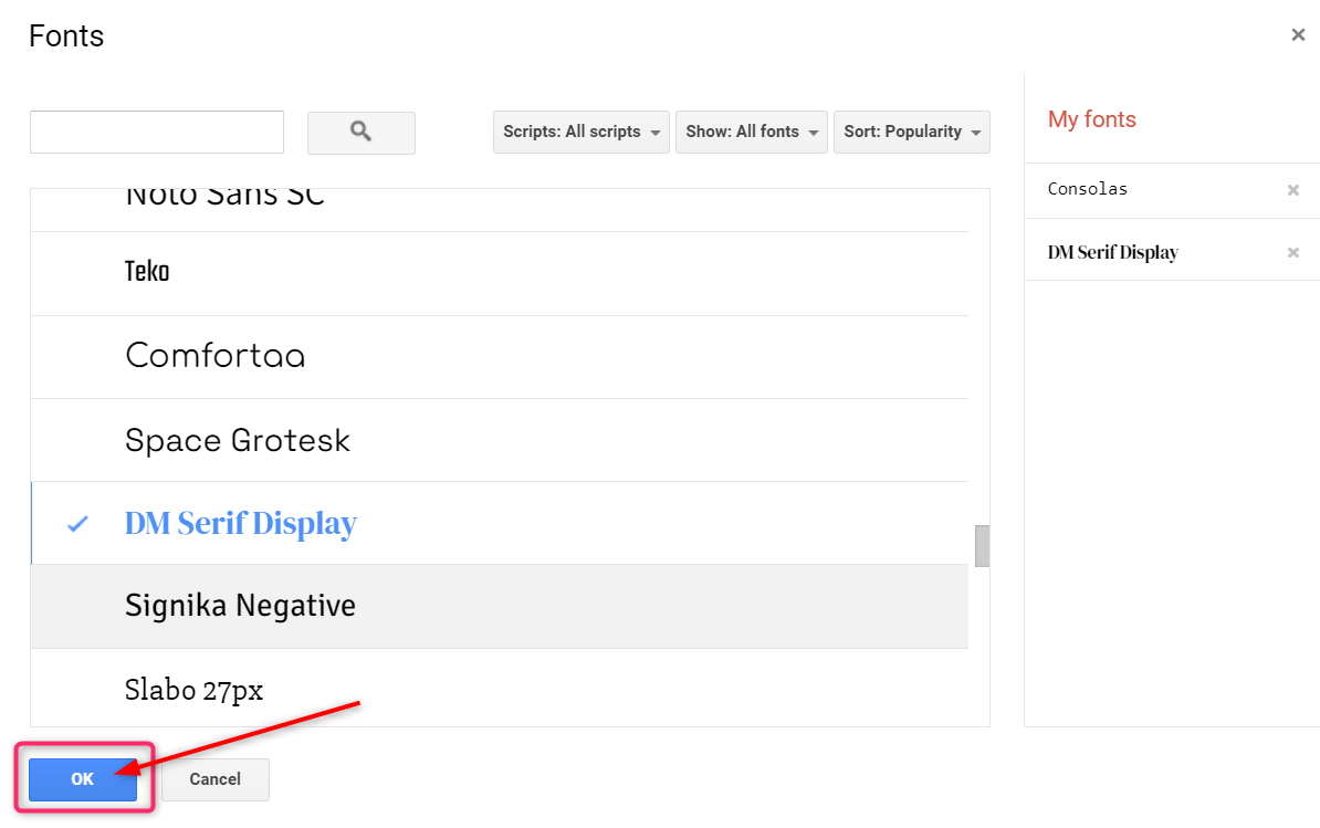
Select the font from the list you wish to add and click on OK:
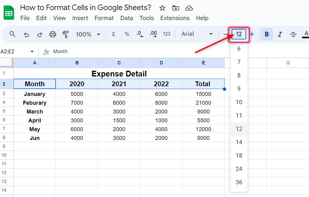
How to Format Cells by Changing Font Size
Changing the font size in Google Sheets helps users read and understand the data more clearly. In order to change the font style, select the cells on which you wish to change the font style, and then click on Font Size options in the toolbar and choose the size from the dropdown you wish to apply on the selected cells:
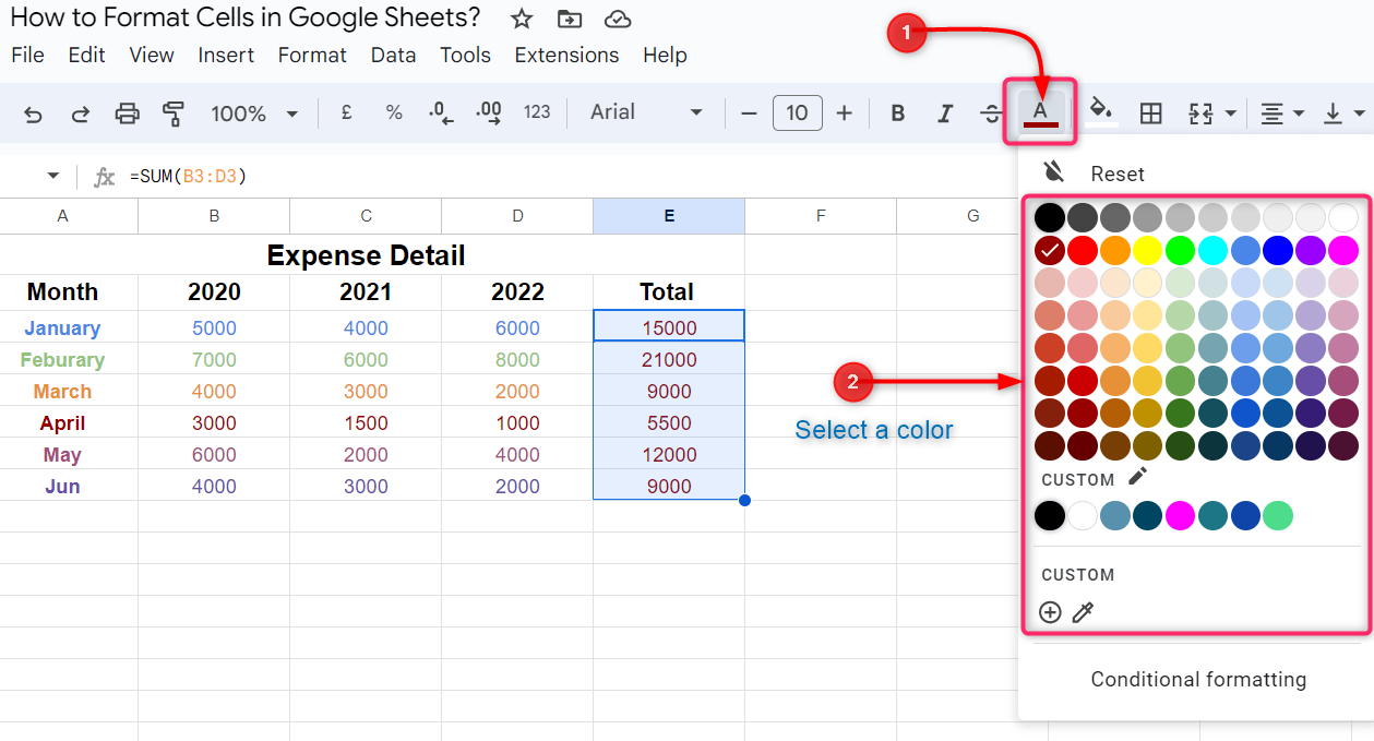
How to Format Cells by Changing Font Color
Changing the text color in cells, differentiating it from the other cells, and helping the reader to understand which type of data is inside specific cells.
Select the cells on which you want to change the text color and click on the Text Color option in the toolbar, then choose a color you wish to apply in the selected cells:
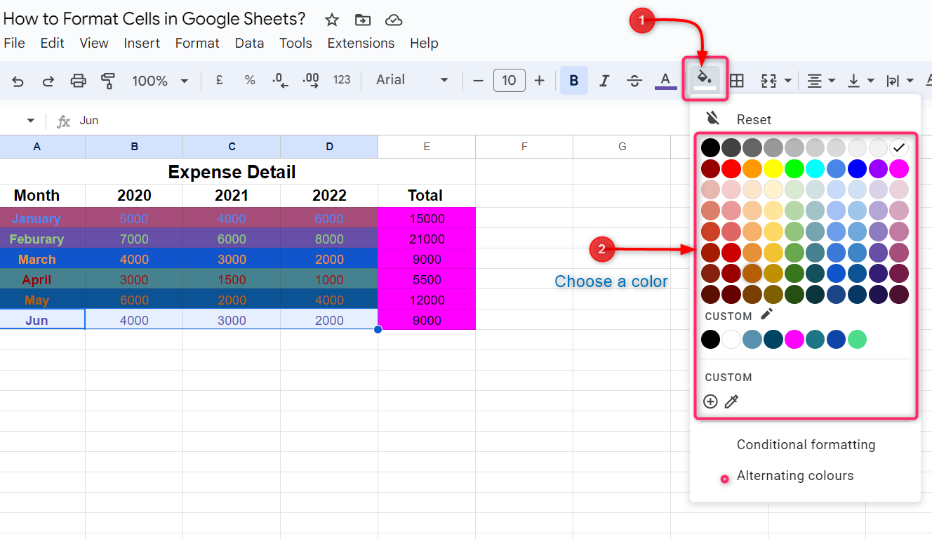
How to Format Cells by Changing Fill Color
Filling color in cells is very useful when you want to differentiate different types of data in a single spreadsheet. It helps the reader to visually understand what type of data is inside the specific colored cells.
To fill color in cells, select the cell you want to fill with color and click on the Fill Color icon in the toolbar. Choose a color from the dropdown, this will automatically apply to the selected cells:
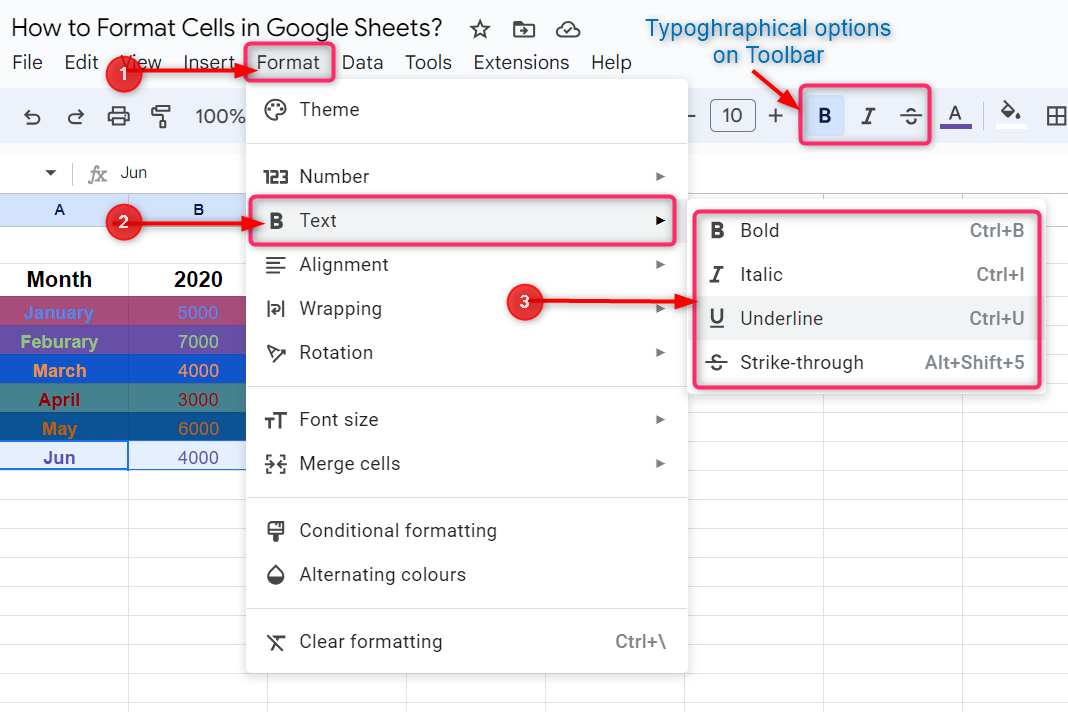
How to Format Cells by Typographical Emphasis
Applying the typographical emphasis gives additional style to the text in the cells. It changes the impact of the words in the cells and helps to differentiate it from the other cells.
There are four types of typographical emphasis you can apply to the texts in the cells on Google Sheets, Bold, Italian, strike-through, and Underline.
To apply the typographical emphasis on cells, select the cells and click on the typographical options you want to apply in the toolbar. This will automatically apply as soon you click on the option. There are only three typographical options available on the toolbar.
To show more options, click on Format and go to Text from the dropdown, and then choose the typographical emphasis you want to apply on the selected cell:
How to Format Cells by Changing Cell Sizes
To keep the text fit into the cells, we need to alter the size of the cells in Google Sheets. There are some simple steps through which you can change the cell’s size.
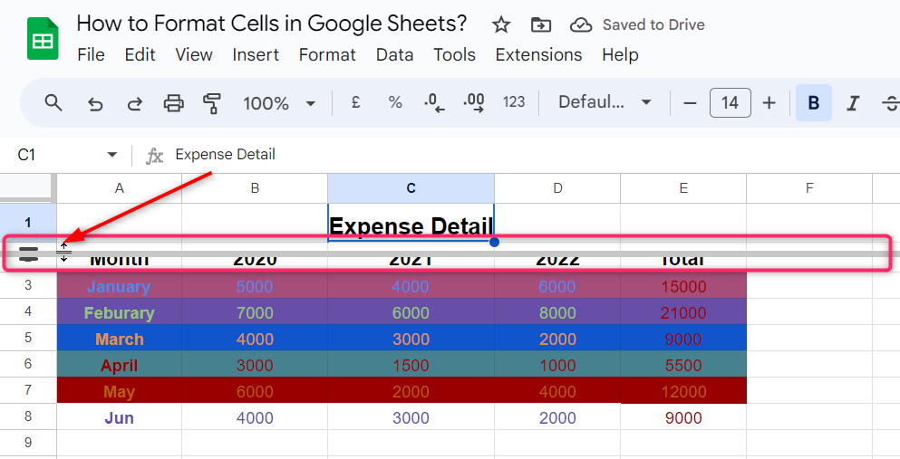
Step 1: Move the Cursor to the Column or Row’s Intersection
Depending on how you wish to alter the cell size, whether horizontally or vertically, move the cursor to the cell’s column intersection or row’s intersection point, respectively. Your cursor will be changed to two vertical lines as shown:
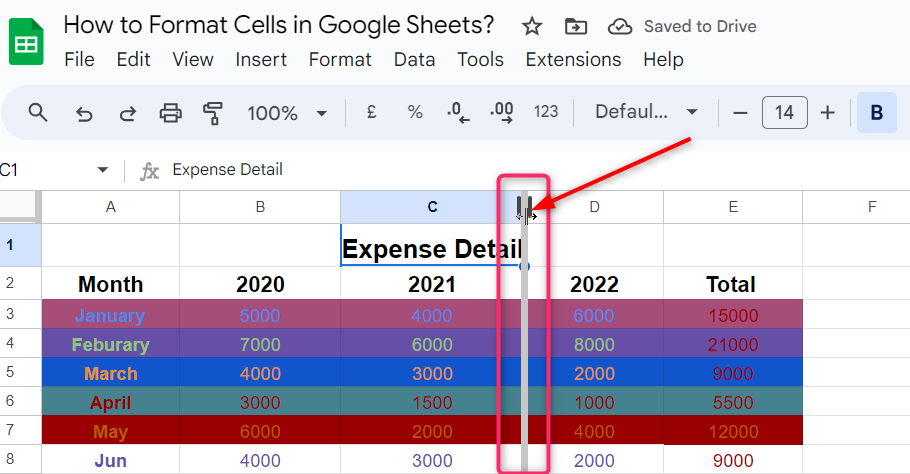
Step 2: Move the Cursor Left or Right
Now move the cursor left or right when you are trying to alter the size horizontally.:
Similarly, to alter the cell size vertically, move the cursor on the row’s intersection and move it up or down:
Pro Tip:
- To alter the cell’s size vertically or horizontally, move the cursor to the column or row intersection where the next column or row starts. Don’t move the cursor at the column or row intersection where the previous column or row ends.
- This will change the size of all the cells inside the column or row.
How to Format Cells by Adding Cell Borders
Adding borders on the cells separates them from the other cells and helps the reader to visually understand them more clearly.
To add borders on the cell in the Google Sheets, select the cells on which you want to add borders and click on the Border icon on the toolbar, then choose the type of border you want to apply on the selected cells from the dropdown:
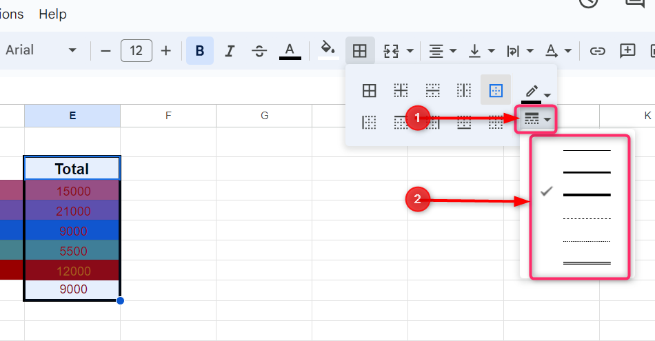
How to Change Border Thickness
To change the border thickness, select the cells for which you want to change the border thickness and open the border dropdown menu as mentioned above. Click on the Thickness icon and select the thickness size from the dropdown:
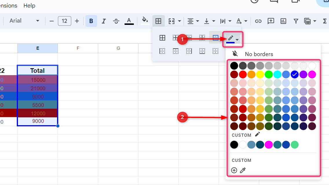
How to Change the Border Color
To change the border color, select the cells and open the border dropdown menu from the toolbar as mentioned above and click on the Pencil icon and select the color from the dropdown:
How to Format Cells by Data Formatting in Cells
Data formatting in cells helps us to properly represent the data values in Google Sheets. There are some ways through which we can format number values in cells.
- Format Numbers Using Local Currency
- Format Numbers Using Custom Currency
- Format Cells Using Date Formatting
- Format Cells Using Time Formatting
1: Format Numbers Using Local Currency
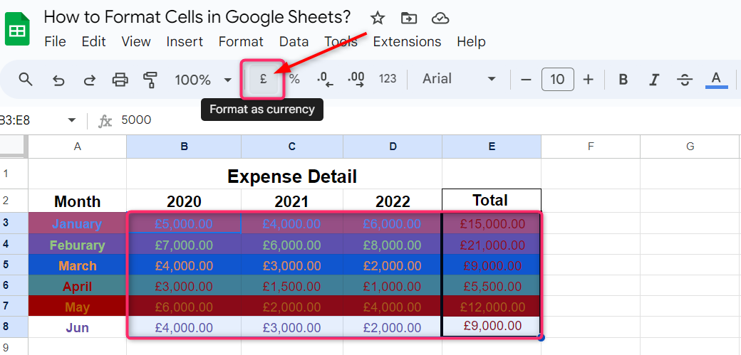
Most of the time, we need to insert financial information in Google Sheets, which requires currency format before the value in the cells.
Select the cells on which we want to apply the local currency format and click on the local currency icon from the toolbar. This will automatically add currency format before the number values in the selected cells:
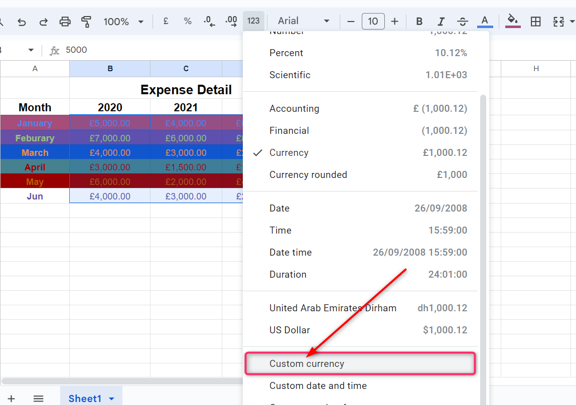
2: Format Numbers Using Custom Currency
As you see, there is only one currency format option on the toolbar, which is according to our local currency. To add non-local or custom currency format on number values in the cells, click on the Number icon on the toolbar and select Custom currency from the dropdown:
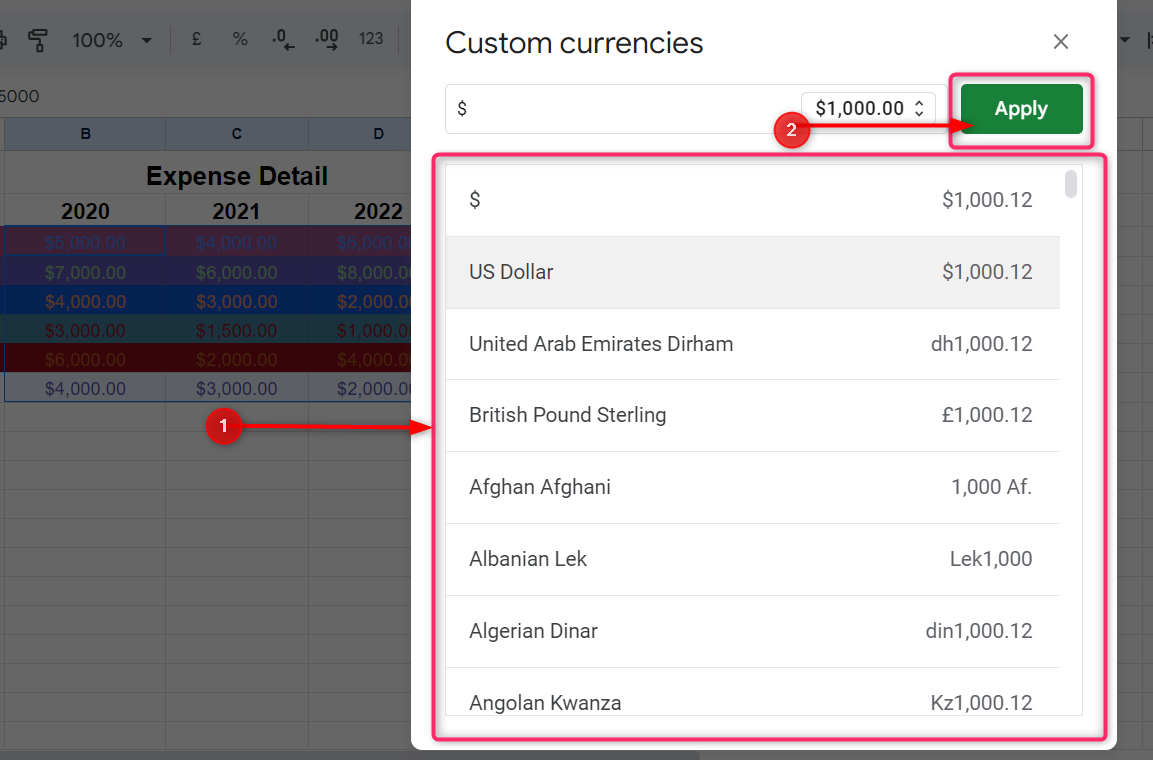
A pop-up window will be open next. Select a currency format you want to apply on the selected cells and click on Apply at the top right of the window:
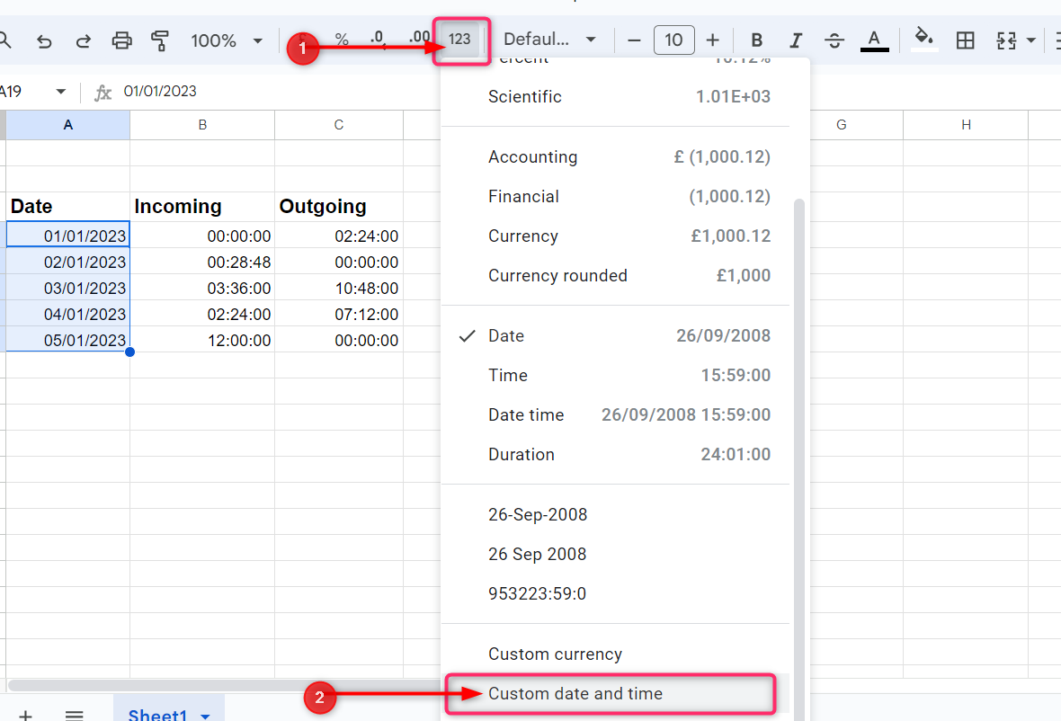
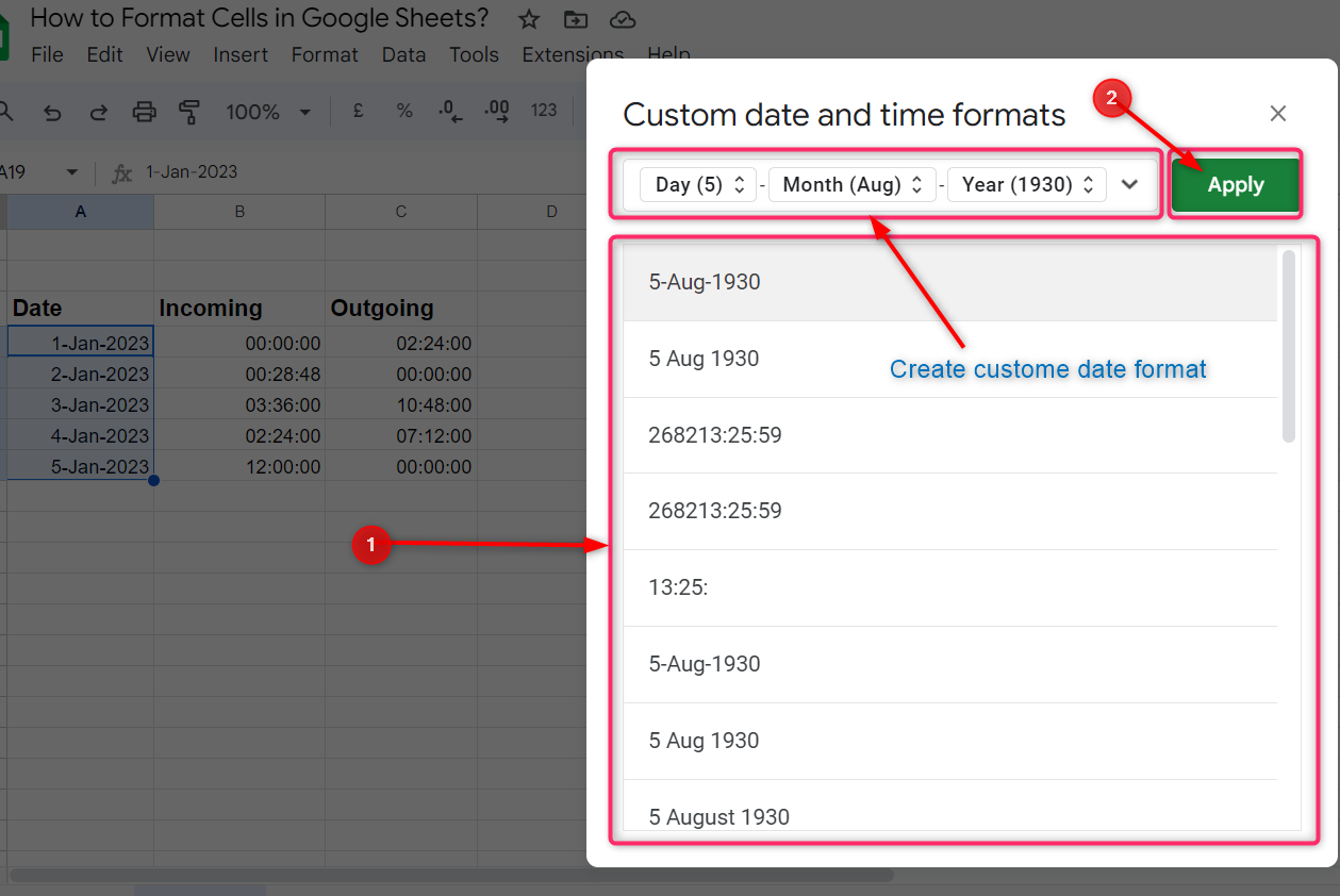
3: Format Cells Using Date and Time Formatting
Most of the time, we have data in the form of dates and times. Google Sheets has built-in dates and time formats to show dates and times in our data more clearly.
To change the date format in Google Sheets, select the cells containing dates and click on the Number icon on the toolbar, then click on Custom date and time from the dropdown:
A pop-up window will open next, where you can select any of the available date formats or create a custom date format and click on Apply at the top right of the pop-up window:
Similarly, we can customize the time format in Google Sheets, select the cells containing the time information and go to Custom date and time as mentioned above. Select the time format from the pop-up window or make a custom time format and click on Apply at the top right of the pop-up window:
Conclusion
To make data in Google Sheets more understandable and presentable, Google Sheets has very useful cell formatting tools. With the use of these cell formatting tools, we can change text color, font size, and font style. We can add a border over the specific data and fill color in the cells to visually understand and differentiate specific data from the other data in Google Sheets. In addition to that, we can add currency format as well as date and time format to the cells that contain the financial information and time and date information in Google Sheets.
Frequently Asked Questions
How can I change the font style in Google Sheets?
To change the font style in Google Sheets, select the cells you want to modify and choose a font style from the dropdown menu under Default (Arial) in the toolbar.
What are the steps to format cells by changing font size in Google Sheets?
To format cells by changing font size in Google Sheets, select the desired cells and adjust the font size using the options available on the toolbar.
How do I change font color in Google Sheets for better visibility?
To change font color in Google Sheets, select the cells you want to modify and choose a color from the font color options in the toolbar.
How to format cells by changing fill color in Google Sheets?
To change fill color in Google Sheets, select the cells you want to format and choose a color from the fill color options available on the toolbar.
What is typographical emphasis and how can I use it to format cells in Google Sheets?
Typographical emphasis is used to highlight text in Google Sheets. To apply typographical emphasis, select the text and choose options like bold, italic, or underline from the toolbar.
How can I adjust cell sizes in Google Sheets to improve readability?
To adjust cell sizes in Google Sheets, select the cells you want to resize and drag the border of the cell to the desired width or height.
What is the importance of adding cell borders in Google Sheets?
Adding cell borders in Google Sheets helps in visually organizing data. To add borders, select the cells and choose the border style and color from the toolbar.
How can I format cells by applying data formatting in Google Sheets?
To format cells by applying data formatting in Google Sheets, select the cells containing data and choose options like number format, date format, or currency format from the toolbar.