
Binary classification means that the output field of the data contains only two classes. It is a supervised learning model that predicts the future in one of two classes: Yes/No, True/False, and others. Logistic Regression is one of the binary classification models to get the categorized output values. The model’s performance is evaluated on metrics like loss, Precision, etc. to optimize its prediction accuracy.

The above image displays the binary classification predictions as the model simply has to place the values above or below the line. Loss values are evaluated on the performance of predicted values as how accurately the values are placed in the correct class. We have one circle present in Class B which indicates the wrong prediction and it increases the loss value of the model. To get the optimized value, we need to get the loss value as low as possible.
Note: The loss value can never be zero as the machine can never observe the external factors, so we make the loss value as close to 0 as it can get.
How to Calculate Loss of Binary Classification Model in PyTorch
Binary classification is used when the client does not require minor details like numerical values. The user needs to set the threshold so the model can predict if the value is above or below the threshold.
To calculate the loss of the binary classification model, build the Logistic Regression, Decision Tree, or any other model. After that, get the dataset and train the model on the given values to predict the future based on the test dataset. The test dataset is usually extracted from the original data and kept hidden from the model to get authentic predictions. To learn the process in detail, simply go through the following steps:
Step 1: Importing Libraries
The first step in this process is importing libraries to get the dependencies or functions to train and test the Logistic Regression model:
import torch
from sklearn.datasets import make_blobs
from matplotlib import pyplot- Import torch library which can be used to get the tensors for storing the binary classification dataset.
- Get the make_blobs library from the datasets dependency and use it to build the binary classification data.
- Import the pyplot library from matplotlib which is used to design the graphical representations for the model’s performance.
Step 2: Building Dataset
The make_blobs() method generates the data in multiple classes to make the dataset appropriate for the classification. Now, use the make_blobs() method to get the training data for the model using the following code. :
x, y = make_blobs(n_samples=[200, 200], random_state=2, cluster_std=1.4, n_features=2)
#splitting data points in two variables as train and test
train = torch.from_numpy(x).type(torch.FloatTensor)
test = torch.from_numpy(y).type(torch.FloatTensor).reshape(-1, 1)
test- Start the process by creating the x and y variables to store the datasets with 200 samples in each variable.
- Arguments in the make_blobs() method are random_state to randomize the values with a standard deviation value of 1.4.
- Here, the n_features argument contains 2 values referring to the binary classification problem and its value can be increased making it multi-classification.
- Now, split the dataset into training and testing samples to use them for model training and then test on the unseen data.
- With that, also normalize the test data in two classes or values using the reshape() method with range.
- Finally, the following screenshot displays the test dataset after normalization containing 0 and 1 values:

Step 3: Designing Logistic Regression
Build the Logistic Regression model using the neural network library of the PyTorch framework with loss and optimizer methods. The Logistic Regression is a binary classification model as it generates the prediction in one of the two given classes:
class LogisticRegression(torch.nn.Module):
  def __init__(self): # Model building in the constructor
    super(LogisticRegression, self).__init__()
    self.linear = torch.nn.Linear(2, 1) # Two input features and one output

  def forward(self, x): # Feed-forward using a linear model to predict
    pred = self.linear(x)
    return torch.sigmoid(pred) # sigmoid activation function on predictions

model = LogisticRegression()
optimizer = torch.optim.SGD(model.parameters(), lr=0.01) #SGD optimizer with arguments
criterion = torch.nn.BCELoss() #get the loss value using the BCELoss() method- Start building the model by creating a class named LogisticRegression with a constructor and forward method.
- Here, the constructor uses the Linear() method to design the flow of the model.
- The forward() method uses the activation function at each process.
- Finally, store the LogisticRegression class in the model variable to easily use it in the training process.
- Then, call the SGD() optimizer for learning data using the models’ parameters.
- In the end, create the criterion variable to call the BCELoss() method to calculate the loss value for the binary classification.
Step 4: Training the Model
After building the model, get to the training phase of the model building to get the most accurate predictions using the epochs as iterations:
for epoch in range(5000):
  pred = model(train) #get predictions from training data
  loss = criterion(pred, test) #get loss value by evaluating the prediction and test values
  loss.backward() #backward propagation
  optimizer.step()
optimizer.zero_grad() #applying the gradient descent- For loop with the epoch variable is used to control the number of iterations while training the model.
- The training process generates predicted values with each iteration and stores them in the pred variable.
- After that, using the loss value is useful in training the model backward to dig deep into the dataset and find hidden insights.
- Then, the optimizer component is used to take the model closer to the prediction and place the value at its proper class.
- Finally, the gradient descent takes large steps at first and keeps getting them down to get the desired prediction.
Step 5: Getting the Model’s Parameters
Now, use the for loop to get the model’s parameters that are used in the training process so the model can be tested using them:
for name, parameter in model.named_parameters():
  print(name, parameter)
After that, apply the forward(train) method on the model to get the prediction using the training data and print the predictions on the screen:
y_pred = model.forward(train)
print(y_pred[:10])
The following screenshot displays the predicted values ranging from 0 to 1:

The required output should be in binary class(2 classes) so simply convert them with 0s and 1s classes:
Step 6: Get the Desired Output
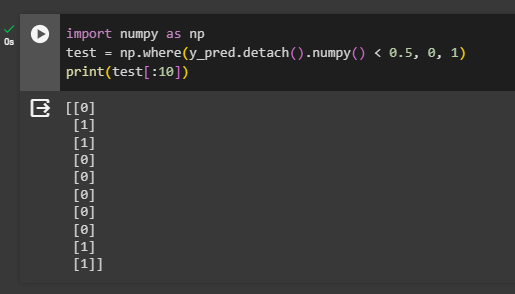
To change the numerical values into categorical format, import the numpy library and set a threshold to classify each value. It allows the model to simply predict and place them in one of the categories made through the threshold:
import numpy as np
test = np.where(y_pred.detach().numpy() < 0.5, 0, 1)
print(test[:10])- The threshold here is set at 0.5 and all the values below this are considered 0 and above are 1.
- Print 10 values from the predicted dataset to check if all the values are according to our choice:
Step 7: Displaying Results
Once we have the values in the required structure, display them in the graphical representation using the following code:
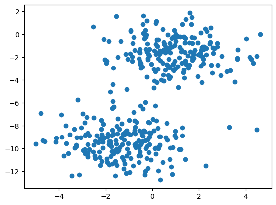
pyplot.scatter(train[:, 0], train[:, 1])- Use the pyplot library to call the scatter() method with the names of the variables to plot the data points.
The following picture displays all the values predicted by the model in a single color.
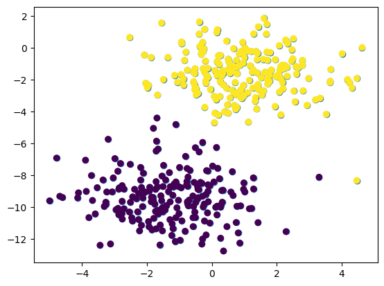
Now, make the representation more interesting by adding colors to each class Both classes are represented with different colors to differentiate them from one another and make the predictions more understandable:
pyplot.scatter(train[:, 0], train[:, 1], c=test)- Adding a “c” argument with the data points from the test variable adds colors to differentiate both classes:
Step 8: Calculating Loss Value
Finally, use the loop to calculate the loss value for each training iteration and print the loss values with its evolution through these iterations:
all_loss = []
for epoch in range(5000):
  pred = model(train)

  loss = criterion(pred, torch.FloatTensor(test))
  all_loss.append (loss.item())
  loss.backward()

  optimizer.step()
  optimizer.zero_grad()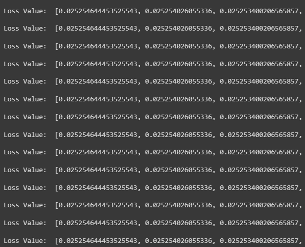
print("Loss Value: ", all_loss)- Firstly, create a list all_loss to calculate the loss value while training the model throughout epochs.
- Now, get the predicted values while training in the pred variable and calculate the loss for each prediction using the criterion variable.
- Then, use the append() method with the all_loss list to store the list of each loss value.
- At the end, print the values of loss for each iteration as shown in the following screenshot:
Step 9: Plotting the Loss Value
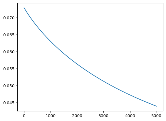
In the end, use the pyplot API of the matplotlib library to create a line graph using the loss values of each iteration. The purpose of multiple iterations is to minimize the loss value to improve the performance of the model:
pyplot.plot(all_loss)The line suggests that the loss values decrease with the epochs starting from more than 70% to below 45%. This shows the improvement in the performance of the model as the model gets trained:
That’s all about the process of calculating the loss of the binary classification model in PyTorch.
Conclusion
To calculate the loss value of the binary classification model, build a binary classification model from multiple options like Naive Bayes, LogisticRegression, etc. Select the model according to the dataset and build its structure to train the model using the existing data. After that, use multiple iterations for training the model to get the predicted values in their classes and check their loss values. Multiple iterations should reduce the loss value and the aim is to make it closer to 0.